Despite representing two third of the European Orthoptera biodiversity, bush crickets (Ensifera: Tettigoniidea) remain often difficult to observe and study in the field. In this article, I will share some personal experiences and highlight potential for future research.

Bush crickets are very distinctive insects. Unlike grasshoppers, which are mainly diurnal, prefer herbaceous vegetation and sing in the audible range, for Tettigoniidea:

– Most species are nocturnal and difficult to detect during the day.

– Many prefer shrubby or woody vegetation and are more difficult to observe in habitats that are difficult to access.

– Most of their songs are high-frequency, at least partly in the ultrasonic range, and are therefore barely or not at all audible to the human ear.

For all these reasons, the use of an ultrasound detector becomes quickly essential when you want to study this group of Orthoptera.

Over the years, I made several thousand recordings of all the species present in the French fauna and many of the Iberian species, both in the field and in captivity, with different temperature conditions for the greatest number of individuals and different localities.

Identification key based on sounds

Thanks to this large library, I was able to measure standard bioaccoustic variables in a systematic way (the dominant frequency, number of syllables, echemes, etc., the duration of syllables, echemes, etc.) and build up a database with each species I could study. Then, I started to search for discriminating criteria between the various species and construct an acoustic identification key and a determination guide to be published in 2025.

The importance of temperature

The differentiation of certain species requires precise measurements, sometimes linked to temperature conditions. This is the case, for example, with the different species of the genus Pholidoptera, where measuring the duration of echemes as a function of temperature enables us to differentiate between 3 acoustically very similar species.

The discovery of species new to science

Acoustic research using an ultrasound detector can also reveal cryptic species that are morphologically very similar. This was the case, for example, for Phaneroptera laticerca, a species widely distributed in the Iberian Peninsula and southern France, but long confused with Phaneroptera nana, which is morphologically very similar. Acoustically, however, the 4 species present in Spain are quite distinct, and each has its own particular characteristics. Their morphological identification in the field remains complicated and is mainly based on the shape of the male cerci, but the progress of acoustic surveys using an ultrasound detector is gradually making it possible to refine our knowledge of their ecology and distribution.

Caractérisation acoustique des différentes espèces du genre Phaneroptera Audinet-Serville, 1831 en Europe occidentale, et description d’une nouvelle espèce cryptique en France et en Espagne (Orthoptera, Tettigoniidae, Phaneropterinae). Zoosystema 43 (29): 691-727. 2021.

Improved detection of shy species

The same work is being carried out on other groups of little-known Iberian species, such as the genera Antaxius and Pterolepis, which are difficult to detect visually and for which acoustic studies seem to provide interesting criteria for gaining a better understanding of their systematics, biology, ecology and evolution.

Miguel Domenech Fernández is a young Spanish orthopterologist based in the province of Albacete. He has been very active since his final year thesis and has gradually incorporated bioacoustics into his research methods. He shares his reflections on his development with us.

_

How did you discover your interest in insects?

From a very young age, practically from the age of 5 or 6, whenever I went to the countryside with my parents, I would carry a container in which I would collect all the insects I saw. Every summer, I would go with my family on vacation to the village (Siles, Jaén), deep in the Segura Mountains. There, I discovered a passion for insects and thoroughly enjoyed observing and searching for them.

_

_

What were your formative stages and what especially attracted you to studying orthoptera?

I studied Biology at the University of Murcia, although professionally I work in the railway sector. From the beginning, I had a keen interest in zoology, geology, and botany, and I disliked laboratory subjects, which took up almost the entire degree (biochemistry, genetics, immunology, physiology, etc.). In recent years, and influenced by both Juan José Presa, who was my professor and tutor for my final project, and David Llucià, I decided to focus my interest on Orthoptera, as it’s a group easy to see on any field trip (not so easy to study) and about which we have little knowledge, generally speaking, in the Iberian Peninsula. Another great passion is mantises, to which I dedicated my final project before specializing in Orthoptera.

What geographic area is your investigation in?

Basically, on the Iberian Peninsula, and within it, in my area of ​​influence, which we could define as the southeastern part of the peninsula. I am and live in Albacete, although I have moved to various parts of the country for work and studies. Given that the province of Albacete doesn’t have many faunal studies on Orthoptera, much less Castilla-La Mancha or nearby areas (such as Jaén), it was interesting to study this area in greater depth, close to me, to try to fill in those information gaps and, of course, enjoy the variety of landscapes that nature delights us with. Both Albacete and most of the neighboring provinces have a great diversity of habitats, making them very interesting for entomology.

_

_

Can you tell us about some of the most interesting species or discoveries?

Beyond having found unrecorded species for several of these provinces or having filled in some gaps in faunal information, I think the most interesting part of my journey has been describing new species. I remember the first, Antaxius oretanus, from Montes de Toledo, thanks to which I was able to strengthen ties with researchers from the MNCN, thus expanding my circle. I then fondly recall some taxa I dedicated to friends of mine, great lovers of entomology in particular and nature in general: Ephippigerida fernandezi, dedicated to Alonso, or the new subspecies I included in the revision of the genus Coracinotus: C. notarioi lluciapomaresi, dedicated to David Llucià, and C. notarioi garciasaucoi, dedicated to Guillermo García-Saúco. Last but not least, in my last published review of the subgenus Bradygaster, I describe Pycnogaster rosae from Cabo de Gata (Almería), dedicating it to my beloved mother, Rosa. I have also given several talks, one on basic bioacoustics at the SEACAM (Environmental Entomological Society of Castilla-La Mancha) conference, and one on Saga pedo, during a special trip to see this species in Albacete organized by the Iberozoa association. I am currently working on updating the information on some species in the Red Book of Endangered Invertebrates of Spain.

_

_

Tell us how you’ve incorporated bioacoustics into your research.
I became interested in bioacoustics after reading various works on Pamphagidae and Bradyporinae, which already covered this subject. I bought Ragge & Reynolds’ book, a great reference for anyone new to orthopteran bioacoustics, and from there I continued reading and reading, also becoming interested in other groups. Then I began making my own recordings, first in the field and then at home using captive specimens. We all associate song with orthopterans (quiet summer nights listening to crickets, for example), and when you begin to study it in depth, you discover many interesting things about their ways of communicating. In Gomphocerinae, for example, there are very specific types of song for each situation (courtship, proclamation, rivalry, etc.). You also discover how each song can vary depending on the ambient temperature, and you begin to learn the typical patterns of each species, with their corresponding intraspecific variability. It’s not a simple discipline, but with interest and enthusiasm, one learns and improves over time. I use a Zoom H4n recorder and subsequently analyze the recordings using editing software (frequently Avisoft), comparing the results with available data published by other authors, if they exist. In most cases, bioacoustics is a complementary tool, sometimes the primary one, with great value when characterizing Orthoptera taxa. There are many cases where taxa are difficult to separate morphologically, but the bioacoustic differences are clearly defining.

_

Being interested in the tiny, in things that can go unnoticed, going out into the countryside and hearing grasshoppers sing isn’t a coincidence; it serves a purpose. When you start to follow the thread and read, to investigate, to ask yourself questions like why, how, when, where… interest is born. A big problem I see is that there are hardly any people interested in these topics, and there must be continuity in the future. Going out into the countryside, beyond serving as a way to disconnect, can allow an amateur to specialize; we all started there. Then there are many hours of reading and studying, but when it’s done out of interest, and not forced upon us, it’s truly very pleasurable, even more so when you can see results you hadn’t imagined. And the advantage of this study is that it can, and should, be combined with the countryside; an outing to connect with nature fills us with peace and a desire to continue.

The Greek workshop has been launched, and a shortlist of 22 participants from 10 countries has been approved.

bc.lab.uoi.gr/en/education-training/teoss/

We have added the recent talk by David Bennet to our canal.

Artículo científico: Recent technological developments allow for passive acoustic monitoring of Orthoptera (grasshoppers and crickets) in research and conservation across a broad range of temporal and spatial scales.

https://www.sciencedirect.com/science/article/pii/S1439179125000258

[et_pb_section fb_built=»1″ _builder_version=»4.16″ custom_margin=»0px|0px|0px|0px|false|false» custom_padding=»0px|0px|0px|0px|false|false» locked=»off» collapsed=»off» global_colors_info=»{}»][et_pb_row _builder_version=»4.16″ background_size=»initial» background_position=»top_left» background_repeat=»repeat» global_colors_info=»{}»][et_pb_column type=»4_4″ _builder_version=»4.16″ custom_padding=»|||» global_colors_info=»{}» custom_padding__hover=»|||»][et_pb_text _builder_version=»4.25.1″ _module_preset=»default» text_font_size=»20px» text_line_height=»1.8em» text_orientation=»justified» locked=»off» global_colors_info=»{}»]

In 2025, we will have a second TEOSS meeting in Spain, but this time we will serve a more international audience with the attendance of participants in the training workshops in 2024. The objective will be to put the TEOSS protocol into practice in the field, searching for the more species the better.

[/et_pb_text][et_pb_image src="https://aeaelbosqueanimado.org/wp-content/uploads/2025/02/Diapositive4.jpg" alt="Taller TEOSS en Verona" title_text="Diapositive4" url="https://docs.google.com/forms/d/e/1FAIpQLSf8SrdPXe_WnqCLsCbbbPIISjZRFJDQJwbteUBYXoJgU3Nw1Q/viewform?usp=header" url_new_window="on" _builder_version="4.25.1" _module_preset="default" hover_enabled="0" global_colors_info="{}" sticky_enabled="0"][/et_pb_image][et_pb_text _builder_version="4.25.1" _module_preset="default" custom_margin="||21px|||" custom_padding="||2px|||" hover_enabled="0" global_colors_info="{}" sticky_enabled="0"]

Inscription

Link.

[/et_pb_text][/et_pb_column][/et_pb_row][/et_pb_section]

[et_pb_section fb_built=»1″ _builder_version=»4.16″ custom_margin=»0px|0px|0px|0px|false|false» custom_padding=»0px|0px|0px|0px|false|false» locked=»off» collapsed=»on» global_colors_info=»{}»][et_pb_row _builder_version=»4.16″ background_size=»initial» background_position=»top_left» background_repeat=»repeat» global_colors_info=»{}»][et_pb_column type=»4_4″ _builder_version=»4.16″ custom_padding=»|||» global_colors_info=»{}» custom_padding__hover=»|||»][et_pb_text _builder_version=»4.25.1″ _module_preset=»default» text_font_size=»20px» text_line_height=»1.8em» text_orientation=»justified» hover_enabled=»0″ locked=»off» global_colors_info=»{}» sticky_enabled=»0″]

THE TEOSS Spain project announces its 2025 meeting in the Serranía de Cuenca on the dates of July 17 to 19, 2025. We will review concepts from the 2024 training workshop and above all we will train data collection in the field.

[/et_pb_text][et_pb_image src="https://aeaelbosqueanimado.org/wp-content/uploads/2025/02/Diapositive3.jpg" alt="Taller TEOSS en Verona" title_text="Diapositive3" url="https://docs.google.com/forms/d/e/1FAIpQLSdljZ1ihi_UtjGQfNbTzNiLyFSyweUDtlCZ9no9RuJpO0jIPQ/viewform?usp=sharing" url_new_window="on" _builder_version="4.25.1" _module_preset="default" global_colors_info="{}"][/et_pb_image][et_pb_text _builder_version="4.25.1" _module_preset="default" custom_margin="||21px|||" custom_padding="||2px|||" global_colors_info="{}"]

Formulario de inscripción

Enlace.

[/et_pb_text][/et_pb_column][/et_pb_row][/et_pb_section]

[et_pb_section fb_built=»1″ _builder_version=»4.25.1″ _module_preset=»default» global_colors_info=»{}»][et_pb_row _builder_version=»4.25.1″ _module_preset=»default» global_colors_info=»{}»][et_pb_column type=»4_4″ _builder_version=»4.25.1″ _module_preset=»default» global_colors_info=»{}»][et_pb_text _builder_version=»4.25.1″ _module_preset=»default» text_font_size=»20px» text_line_height=»1.8em» text_orientation=»justified» locked=»off» global_colors_info=»{}»]

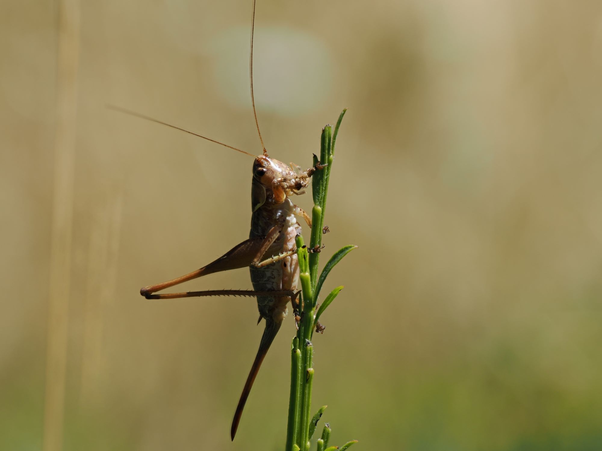
While many invertebrates produce sounds incidentally, cicadas, crickets, and grasshoppers stand out for their ability to produce loud, purposeful sounds that play vital roles in their communication, reproduction, and survival strategies. The male songs are indeed specific to each species and can even be more reliable indicators for identification than morphological characteristics.

[/et_pb_text][et_pb_image src="https://aeaelbosqueanimado.org/wp-content/uploads/2024/09/Eugryllodes-pipiens-paloma.jpg" title_text="Eugryllodes pipiens paloma" _builder_version="4.25.1" _module_preset="default" global_colors_info="{}"][/et_pb_image][et_pb_text _builder_version="4.25.1" _module_preset="default" custom_padding="||50px|||" global_colors_info="{}"]

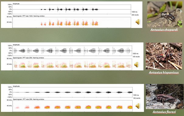
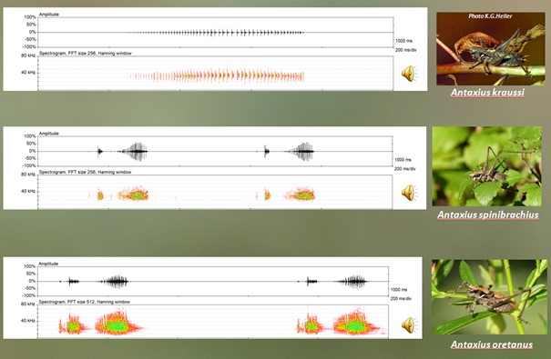
The male’s song is unique to each species and predominantly follows a repetitive and consistent pattern that can be characterized by its tone, volume and rhythm. Graphical representations of these two parameters provide valuable tools for visualizing and analyzing these specific acoustic features, facilitating the comparison of songs across different species or individuals.

[/et_pb_text][et_pb_text _builder_version=»4.25.1″ _module_preset=»default» header_2_text_color=»#8300E9″ custom_padding=»||0px|||» global_colors_info=»{}»]

PART I. SOUND PRODUCTION IN ORTHOPTERA

Sound production in Orthoptera, known as stridulation, is achieved by the movement of specialized sound-producing structures. Fundamentally, a line (file, series) of teeth (serrations, pegs) located in one body part moves against a rigid structure (vein, ridge) located on another body part. Each tooth impact produces a discrete burst of sound energy (= one pulse). As the entire file of pegs impact against the scraper, many pulses are generated which create a complex of sounds.

[/et_pb_text][et_pb_text _builder_version=»4.25.1″ _module_preset=»default» global_colors_info=»{}»]

Ensifera: elytral-elytral stridulation

The sound production mechanism known as elytral-elytral stridulation is characteristic of crickets and bush crickets (Orthoptera: Ensifera). Here are the key points:
[/et_pb_text][et_pb_image src="https://aeaelbosqueanimado.org/wp-content/uploads/2024/10/ENsifera-sound-structures.png" title_text="ENsifera sound structures" _builder_version="4.25.1" _module_preset="default" global_colors_info="{}"][/et_pb_image][et_pb_text _builder_version="4.25.1" _module_preset="default" text_font="|700|||||||" text_text_color="#0C71C3" custom_margin="-10px||50px||false|false" custom_padding="0px||||false|false" global_colors_info="{}"]

Sound producing structures in Ensifera (Rafael Carbonnel).

[/et_pb_text][et_pb_text _builder_version=»4.25.1″ _module_preset=»default» global_colors_info=»{}»]

1. Involved structures
– Tegmina: The first pair of hardened wings.
– Thickened vein: Located on one of the tegmina (left in Tettigoniidae, right in Gryllidae).
– Posterior margin: Of the opposite tegmina.

2. Mechanism
– The tegmina rub against each other in a scissor-like motion.
– The scraper (thickened vein) rubs against the file (posterior margin) of the other tegmen.
– Typically, the sound is produced during the closing movement of the tegmina.

3. Variations
– The duration of the closing movement can vary significantly among species:
– Uromenus rugosicollis: 0.4 seconds (up to 2 seconds on cold nights)
– Ruspolia nitidula: Up to 100 closures per second

This mechanism allows Ensifera to produce species-specific calls that are essential for intraspecific communication, particularly in mating and territorial contexts. The variation in the speed and pattern of stridulation contributes to the acoustic diversity observed within this group of insects.

[/et_pb_text][/et_pb_column][/et_pb_row][et_pb_row _builder_version=»4.25.1″ _module_preset=»default» global_colors_info=»{}»][et_pb_column type=»4_4″ _builder_version=»4.25.1″ _module_preset=»default» global_colors_info=»{}»][et_pb_text _builder_version=»4.25.1″ _module_preset=»default» global_colors_info=»{}»]

Caelifera: leg-to-elytral stridulation

Sound production mechanism in grasshoppers (Orthoptera: Caelifera) involves a completely different system:

[/et_pb_text][et_pb_image src="https://aeaelbosqueanimado.org/wp-content/uploads/2024/10/Caelifera-sound-structures.png" title_text="Caelifera sound structures" _builder_version="4.25.1" _module_preset="default" global_colors_info="{}"][/et_pb_image][et_pb_text _builder_version="4.25.1" _module_preset="default" text_font="|700|||||||" text_text_color="#0C71C3" custom_margin="-10px||50px||false|false" custom_padding="0px||||false|false" global_colors_info="{}"]

Sound producing structures in Caelifera (Rafael Carbonnel).

[/et_pb_text][et_pb_text _builder_version=»4.25.1″ _module_preset=»default» global_colors_info=»{}»]

1. Structures involved
– File (raspa): A row of tiny teeth on the inner surface of the hind femur.
– Scraper: A hardened vein on the tegmina.

2. Mechanism
– Friction between the inner surface of the hind femur and a hardened vein on the tegmina (forewings).
– The hind leg pivots up and down, rubbing the file against the scraper.
– This can occur up to 20 times per second, varying by species:
– Minimum: 1 stroke/second in S. lineatus
– Maximum: 120 syllables/second in S. nigrolineatus

4. Dual mechanism
– Grasshoppers have two hind legs, providing a double stridulation mechanism.
– This allows for subtle variations in signal structure by phasing the movement of the legs.

5. Variations in Oedipodinae
In this subfamily, the arrangement is reversed:
– The tegminal vein has teeth
– The femur has a smooth internal ridge
– This produces a weaker sound.

This femur-tegmina friction mechanism is distinct from the elytral-elytral stridulation used by crickets and katydids, showcasing the diversity of sound production methods within Orthoptera. This mechanism allows grasshoppers to produce a variety of sounds by altering speed of leg movement, pressure applied and coordination between legs.

[/et_pb_text][/et_pb_column][/et_pb_row][et_pb_row _builder_version=»4.25.1″ _module_preset=»default» global_colors_info=»{}»][et_pb_column type=»4_4″ _builder_version=»4.25.1″ _module_preset=»default» global_colors_info=»{}»][et_pb_text _builder_version=»4.25.1″ _module_preset=»default» global_colors_info=»{}»]

Other mechanisms in Orthoptera

The Oak bush-cricket (Meconema thalassinum) is unique in its sound production method among European Orthoptera. Instead of using wing-based stridulation, M. thalassinum drums with one of its hind tarsi (feet) on a leaf or branch.

The drumming produces a series of short, percussive sounds. The sound produced (frequency and amplitude) depends on the substrate the insect is drumming on. This results in variable acoustic properties depending on the surface.

[/et_pb_text][/et_pb_column][/et_pb_row][et_pb_row _builder_version=»4.25.1″ _module_preset=»default» global_colors_info=»{}»][et_pb_column type=»4_4″ _builder_version=»4.25.1″ _module_preset=»default» global_colors_info=»{}»][et_pb_text _builder_version=»4.25.1″ _module_preset=»default» global_colors_info=»{}»]

Cicadas: a different insect order = a different sound mechanism

[/et_pb_text][/et_pb_column][/et_pb_row][/et_pb_section][et_pb_section fb_built=»1″ _builder_version=»4.25.1″ _module_preset=»default» global_colors_info=»{}»][et_pb_row _builder_version=»4.25.1″ _module_preset=»default» global_colors_info=»{}»][et_pb_column type=»4_4″ _builder_version=»4.25.1″ _module_preset=»default» global_colors_info=»{}»][et_pb_text _builder_version=»4.25.1″ _module_preset=»default» header_2_text_color=»#8300E9″ global_colors_info=»{}»]

PART II. PARAMETERS TO DESCRIBE SOUNDS IN ORTHOPTERA

The main physical parameters used to analyze and distinguish the songs of different species are:

[/et_pb_text][et_pb_text _builder_version=»4.25.1″ _module_preset=»default» global_colors_info=»{}»]

Tone of an insect song

The frequency of the song refers to the tone or pitch of the sound and is measured in Hertz (Hz). While low pitched sounds produced by Orthopterafall within the hearing of humans, high pitch sounds are inaudible and must be recorded with specific microphones.

Some Orthoptera (crickets and grasshoppers) produce low-pitched sounds that are audible to humans and others (bush-crickets) emit high-pitched sounds that require specialized microphones to detect. Note that insects can produce sounds of different frequencies at the same time that are variable to some extent during the song.

The frequency of sound over time is visually displayed in graphs called spectrograms.

[/et_pb_text][et_pb_image src="https://aeaelbosqueanimado.org/wp-content/uploads/2024/10/Spectogram_.jpg" title_text="Spectogram_" _builder_version="4.25.1" _module_preset="default" global_colors_info="{}"][/et_pb_image][et_pb_text _builder_version="4.25.1" _module_preset="default" text_font="|700|||||||" text_text_color="#0C71C3" custom_margin="-10px||50px||false|false" custom_padding="0px||||false|false" global_colors_info="{}"]

Spectrogram of an Orthoptera sound. X = time. Y = Frequency (kHz). In red, higher amplitudes.

[/et_pb_text][et_pb_text _builder_version=»4.25.1″ _module_preset=»default» global_colors_info=»{}»]

Volume of the sound

Sound amplitude, commonly known as loudness, is expressed in decibels (dB) and represents the intensity or strength of an acoustic signal. Decibels use a logarithmic scale to represent the wide range of sound intensities that the human ear can perceive. The human ear perceives an increase of 10 dB as a doubling of volume.

Of course, the volume of a song is not constant and oscillogram represents the amplitude of the sound as a function of time.
[/et_pb_text][et_pb_image src="https://aeaelbosqueanimado.org/wp-content/uploads/2024/10/oscillogram.jpg" title_text="oscillogram" _builder_version="4.25.1" _module_preset="default" global_colors_info="{}"][/et_pb_image][et_pb_text _builder_version="4.25.1" _module_preset="default" text_font="|700|||||||" text_text_color="#0C71C3" custom_margin="-10px||50px||false|false" custom_padding="0px||||false|false" global_colors_info="{}"]

Oscillogram an Orthoptera sound. X = time. Y = Amplitude (dB).

[/et_pb_text][et_pb_text _builder_version=»4.25.1″ _module_preset=»default» global_colors_info=»{}»]

Rhythm of the song

The rhythm is visible on the oscillogram, especially examining records at very slow motion. Rhythm or repetition rate refers to the temporal pattern of the sounds, generally measured in pulses per second or per minute.

> Echeme is the visible unit of the song pattern

An echeme is a discrete unit of sound production in insect calls. It’s often described as a «chirp» or a «trill» in common language. Echemes are separated by periods of silence and form the basic building blocks of many Orthopteran acoustic signals. Therefore, it can be considered as the basic unit of the song pattern although it is a complex of individual sounds.

[/et_pb_text][et_pb_image src="https://aeaelbosqueanimado.org/wp-content/uploads/2024/10/Echeme.jpg" title_text="Echeme" _builder_version="4.25.1" _module_preset="default" global_colors_info="{}"][/et_pb_image][et_pb_text _builder_version="4.25.1" _module_preset="default" text_font="|700|||||||" text_text_color="#0C71C3" custom_margin="-10px||50px||false|false" custom_padding="0px||||false|false" global_colors_info="{}"]Oscilogram showing a succession of echemes. In red: one echeme.
[/et_pb_text][et_pb_text _builder_version="4.25.1" _module_preset="default" global_colors_info="{}"]

> Syllable is the sounds produced by one complete movement of the stridulatory system

A syllable is the unit of sound production in insect calls corresponding to one complete cycle of wing movement in crickets or one leg stroke in grasshoppers. Syllables are the components that make up echemes.

The following drawing is even slower down and also shows in the top part both legs movement of a grasshopper along a time line, resulting in sound production (displayed here as an oscilogram). A syllable (S) is the unit which represent an entire movement of wings/legs.

[/et_pb_text][et_pb_image src="https://aeaelbosqueanimado.org/wp-content/uploads/2024/10/syllable.jpg" title_text="syllable" _builder_version="4.25.1" _module_preset="default" global_colors_info="{}"][/et_pb_image][et_pb_text _builder_version="4.25.1" _module_preset="default" text_font="|700|||||||" text_text_color="#0C71C3" custom_margin="-10px||50px||false|false" custom_padding="0px||||false|false" global_colors_info="{}"]Slow-down oscilogram, showing a series of syllables (S).
[/et_pb_text][et_pb_text _builder_version="4.25.1" _module_preset="default" global_colors_info="{}"]

> Pulse is one single tooth impact

A pulse is a fundamental unit of sound production, a brief and discrete burst of sound energy produced by a single movement of the finer sound-producing structure (= one tooth stroke).

We can distinguish the duration (D) of the pulses, time that each individual sound lasts within the song, and the intervals (I) between pulses, the time of silence between each sound. Period (P) is D+I.

[/et_pb_text][et_pb_image src="https://aeaelbosqueanimado.org/wp-content/uploads/2024/10/parameter.jpg" title_text="parameter" _builder_version="4.25.1" _module_preset="default" global_colors_info="{}"][/et_pb_image][et_pb_text _builder_version="4.25.1" _module_preset="default" text_font="|700|||||||" text_text_color="#0C71C3" custom_margin="-10px||50px||false|false" custom_padding="0px||||false|false" global_colors_info="{}"]

Slow-down oscilogram, showing the duration (D), interval (I) and period (P) of a pulse.

[/et_pb_text][et_pb_text _builder_version=»4.25.1″ _module_preset=»default» global_colors_info=»{}»]

Revisited spectrogram

Another way to represent a stridulation is to not consider the time as the X axis, but instead analyze the characteristics of the sound during an entire lapse of time. In this case, the frequency is represented against the amplitude, showing quickly which is the dominant pitch during the song.

[/et_pb_text][et_pb_image src="https://aeaelbosqueanimado.org/wp-content/uploads/2024/10/graph-3.jpg" title_text="graph 3" _builder_version="4.25.1" _module_preset="default" global_colors_info="{}"][/et_pb_image][et_pb_text _builder_version="4.25.1" _module_preset="default" text_font="|700|||||||" text_text_color="#0C71C3" custom_margin="-10px||50px||false|false" custom_padding="0px||||false|false" global_colors_info="{}"]

Another spectrogram representation. X = Frequency (kHz) instead of Y axis as in the usual graph. Y = Amplitude.

[/et_pb_text][/et_pb_column][/et_pb_row][/et_pb_section][et_pb_section fb_built="1" _builder_version="4.25.1" _module_preset="default" global_colors_info="{}"][/et_pb_section][et_pb_section fb_built="1" _builder_version="4.25.1" _module_preset="default" global_colors_info="{}"][et_pb_row column_structure="1_2,1_2" _builder_version="4.16" _module_preset="default" locked="off" global_colors_info="{}"][et_pb_column type="1_2" _builder_version="4.16" _module_preset="default" background_color="#efefef" global_colors_info="{}"][et_pb_image src="https://aeaelbosqueanimado.org/wp-content/uploads/2024/04/Tettris-logo.jpg" title_text="Tettris logo" _builder_version="4.16" _module_preset="default" global_colors_info="{}"][/et_pb_image][/et_pb_column][et_pb_column type="1_2" _builder_version="4.16" _module_preset="default" background_color="#efefef" global_colors_info="{}"][et_pb_image src="https://aeaelbosqueanimado.org/wp-content/uploads/2024/04/eu_funded_en.jpg" title_text="Flag_2colors.eps" _builder_version="4.16" _module_preset="default" global_colors_info="{}"][/et_pb_image][/et_pb_column][/et_pb_row][et_pb_row _builder_version="4.25.1" _module_preset="default" locked="off"][et_pb_column _builder_version="4.25.1" _module_preset="default" type="4_4"][et_pb_text _builder_version="4.25.1" _module_preset="default" hover_enabled="0" sticky_enabled="0"]

Funded by the European Union. Views and opinions expressed are however those of the author(s) only and do not necessarily reflect those of the European Union or REA. Neither the European Union nor REA can be held responsible for them.

[/et_pb_text][/et_pb_column][/et_pb_row][/et_pb_section]

[et_pb_section fb_built=»1″ _builder_version=»4.25.1″ _module_preset=»default» global_colors_info=»{}»][et_pb_row _builder_version=»4.25.1″ _module_preset=»default» global_colors_info=»{}»][et_pb_column type=»4_4″ _builder_version=»4.25.1″ _module_preset=»default» global_colors_info=»{}»][et_pb_text _builder_version=»4.25.1″ _module_preset=»default» text_font_size=»20px» text_line_height=»1.8em» text_orientation=»justified» locked=»off» global_colors_info=»{}»]

During TEOSS workshops we will be aiming at collecting Orthopteran sound recordings of well-identified species with a minimum set of metadata. Our aim is to train recorders for making possible automatic species recognition based on sound recordings for a larger part of the European Orthoptera fauna.

[/et_pb_text][et_pb_image src="https://aeaelbosqueanimado.org/wp-content/uploads/2024/07/Recording-with-a-Tascamx40.jpg" alt="Recording with a Tascamx40" title_text="Recording with a Tascamx40" _builder_version="4.25.1" _module_preset="default" global_colors_info="{}"][/et_pb_image][et_pb_text _builder_version="4.25.1" _module_preset="default" header_2_text_color="#8300E9" custom_padding="||0px|||" locked="off" global_colors_info="{}"]

PART I. INTRODUCTION. GETTING SOME CONCEPTS.

[/et_pb_text][et_pb_text _builder_version=»4.25.1″ _module_preset=»default» global_colors_info=»{}»]

Recording devices and microphones

During the workshop we will be recording with the following types of devices:
● Good digital recorder with or without external microphone
● Cheap digital recorder using internal microphone
● Phone with ultrasonic microphone
● Phone with non-ultrasonic microphone
● Phone with internal microphone
In combination with using different sample rates, this will yield a great variation in quality of sound recordings. We aim to let every participant use every device, to be able to experience the difference in (technical) handling, ease of use and recording quality.

[/et_pb_text][et_pb_text _builder_version=»4.25.1″ _module_preset=»default» global_colors_info=»{}»]

Minimum recording quality and size

We only will be recording digitally, with a sampling frequency at or above 44.1 kHz (up to 354 kHZ) and bit depth of 16 bits (or maybe 24 bits). We will save our files uncompressed, meaning in WAV-format, so not compressed in e.g. mp3, m4a, aac, flac, or ogg. We must be aware that some analysis software only accepts files with 16-bit depth and that online platforms accept also higher bit depth files (table 1).

[/et_pb_text][et_pb_image src="https://aeaelbosqueanimado.org/wp-content/uploads/2024/11/Handling-of-sound-recordings-on-different-web-platforms.jpg" title_text="Handling of sound recordings on different web platforms" _builder_version="4.25.1" _module_preset="default" global_colors_info="{}"][/et_pb_image][et_pb_text _builder_version="4.25.1" _module_preset="default" text_font="|700|||||||" text_text_color="#0C71C3" custom_margin="-10px||50px||false|false" custom_padding="0px||||false|false" global_colors_info="{}"]

Table 1: Handling of sound recordings on different web platforms.

[/et_pb_text][et_pb_text _builder_version=»4.25.1″ _module_preset=»default» global_colors_info=»{}»]

High quality (stereo) recordings easily become very large. Online platforms accept only small thus short files (except Xeno-canto that accepts 128Mb, see table 2). This means that high-quality sound recordings may last only a few seconds, which may be too short to record the full courtship song of a Gomphocerine grasshopper, for example. This is one of the reasons we decided to go for uploading sound recordings to Xeno-canto (XC) during TEOSS.

[/et_pb_text][et_pb_image src="https://aeaelbosqueanimado.org/wp-content/uploads/2024/11/Maximum-duration-of-sound-recordings-of-different-quality.jpg" title_text="Maximum duration of sound recordings of different quality" _builder_version="4.25.1" _module_preset="default" global_colors_info="{}"][/et_pb_image][et_pb_text _builder_version="4.25.1" _module_preset="default" text_font="|700|||||||" text_text_color="#0C71C3" custom_margin="-10px||50px||false|false" custom_padding="0px||||false|false" global_colors_info="{}"]

Table 2: Maximum duration of sound recordings of different quality, based on maximum file sizes of 10, 20 and 128Mb.

[/et_pb_text][et_pb_text _builder_version=»4.25.1″ _module_preset=»default» text_orientation=»justified» global_colors_info=»{}»]

Metadata

We need to add a minimum set of metadata to the sound recordings. This is important for several reasons:

● When including locality date and coordinates, the sound recording will be shared through GBIF, making the recording available as an observation for research and conservation.

● Including information on the recording device and quality may help to understand the representation of the song in the recording.

● Including temperature and time of day during recording is important to know under what conditions species sing and how song characters may depend on temperature.

[/et_pb_text][/et_pb_column][/et_pb_row][et_pb_row _builder_version="4.25.1" _module_preset="default" global_colors_info="{}"][et_pb_column type="4_4" _builder_version="4.25.1" _module_preset="default" global_colors_info="{}"][et_pb_image src="https://aeaelbosqueanimado.org/wp-content/uploads/2024/07/Recording-in-San-Giorgio-with-an-EchoMeter.jpg" alt="Recording in San Giorgio with an EchoMeter" title_text="Recording in San Giorgio with an EchoMeter" _builder_version="4.25.1" _module_preset="default" global_colors_info="{}"][/et_pb_image][/et_pb_column][/et_pb_row][et_pb_row _builder_version="4.25.1" _module_preset="default" global_colors_info="{}"][et_pb_column type="4_4" _builder_version="4.25.1" _module_preset="default" global_colors_info="{}"][et_pb_text _builder_version="4.25.1" _module_preset="default" header_2_text_color="#8300E9" custom_padding="||0px|||" locked="off" global_colors_info="{}"]

PART II. WORKFLOW IN THE FIELD

[/et_pb_text][et_pb_text _builder_version=»4.25.1″ _module_preset=»default» text_orientation=»justified» global_colors_info=»{}»]

Participants of the workshop will be instructed beforehand about this workflow and how to use the recorders and microphones available. Also, field forms to note metadata and tubes to temporarily collect specimens will be handed out. The workflow in the field has the following steps.

[/et_pb_text][et_pb_text _builder_version=»4.25.1″ _module_preset=»default» text_orientation=»justified» global_colors_info=»{}»]

Reaching the location

● Travel to field location. Note Metadata: COUNTRY / PROVINCE / MUNICIPALITY / LOCALITY.
● Hand out recorders Note Metadata: RECORDER/MICROPHONE.
● Attend instructions before field work (e.g. on the time to be back or species to expect or search for).
● Synchronize date/time between Digital Recorder / Smartphone / Camera. Note Metadata: DATE / TIME.
● Basic approach: One sound = one record = one line of data in the paper field form.
● In summary, fieldwork involves 5 successive steps : 1) Recording sounds and 2) taking Pictures and/or 3) collecting the specimen and 4) filling Observation datalog (aka “OBSERVATION”) (using the app Obsmapp or iObs (Observation.org)) and 5) filling the paper form (aka “FORM”).
● Silently participants start to approach carefully singing specimens and start collecting records and note down all relevant metadata. (Note: some metadata may be extracted in the lab from observation.org). Note Metadata: TEMPERATURE and maybe a note if the specimen is in a sunny site or in the shade).

[/et_pb_text][et_pb_image src="https://aeaelbosqueanimado.org/wp-content/uploads/2024/11/Fieldwork-sheet.jpg" _builder_version="4.25.1" _module_preset="default" title_text="Fieldwork sheet" hover_enabled="0" sticky_enabled="0" border_color_all="#0C71C3" border_radii="on|1px|1px|1px|1px" border_width_all="3px"][/et_pb_image][et_pb_text _builder_version="4.25.1" _module_preset="default" text_font="|700|||||||" text_text_color="#0C71C3" custom_margin="-10px||50px||false|false" custom_padding="0px||||false|false" hover_enabled="0" global_colors_info="{}" sticky_enabled="0"]

Fieldwork sheet -ready to download-

[/et_pb_text][et_pb_text _builder_version=»4.25.1″ _module_preset=»default» text_orientation=»justified» global_colors_info=»{}»]

Sound recording procedure

● Step 1: Record one sound sequence (two situations: various sound files with short recordings or only one long sound file).
     o Select a proper recording and note down the name of this recording. Note Metadata: RECORDING NAME.
     o Test various recording setups (close distance with handheld recorder vs long distance with use of stick ; check microphone and recorder options) which generate different records.
     o Note the sound type (calling song, rivalry song courtship song, linked to behavior, Note Metadata: SONG TYPE.

● Step 2: Compulsory, take pictures of the specimen as a way of identifying the species or keeping a voucher of the specimen:
     o With the smartphone (consider to allow the geolocation of images in the smartphone setups);
     o With a dedicated camera (very often, geolocation is not available, look carefully at correct Date and Time setups, especially if you traveled from a different time zones).
     o You could also take a blank picture (e.g. sky) between two consecutive specimens, especially if they belong to the same species, in order to ease lab work.

● Step 3: Eventually, capture the specimen with a net for close-up pictures or for collecting purposes. Collected specimens should be labeled in the field with the date, locality, name of collector (traditional entomology). Add time of recollection and any detail for ease of future referencing in the lab.

● Step 4: Use the phone’s APP (Obsmapp/iobs) to record the observation in the field. If the APP is not used in the field, you will have the possibility to record the observation in the website, back in the lab.

● Step 5: COMPULSORY. Fill the paper form with the sound file name and relevant information that allow you to fill in the lab the projects’ database.

[/et_pb_text][/et_pb_column][/et_pb_row][et_pb_row _builder_version="4.25.1" _module_preset="default" global_colors_info="{}"][et_pb_column type="4_4" _builder_version="4.25.1" _module_preset="default" global_colors_info="{}"][et_pb_image src="https://aeaelbosqueanimado.org/wp-content/uploads/2024/07/Uploading-data.jpg" alt="Uploading data" title_text="Uploading data" _builder_version="4.25.1" _module_preset="default" global_colors_info="{}"][/et_pb_image][/et_pb_column][/et_pb_row][et_pb_row _builder_version="4.25.1" _module_preset="default" global_colors_info="{}"][et_pb_column type="4_4" _builder_version="4.25.1" _module_preset="default" global_colors_info="{}"][et_pb_text _builder_version="4.25.1" _module_preset="default" header_2_text_color="#8300E9" custom_padding="||0px|||" locked="off" global_colors_info="{}"]

PART III. BACK IN THE LAB

[/et_pb_text][et_pb_text _builder_version=»4.25.1″ _module_preset=»default» text_orientation=»justified» global_colors_info=»{}»]

In the lab or hotel room/lobby, the following activities take place, preferably shortly after return from the field:

[/et_pb_text][et_pb_text _builder_version=»4.25.1″ _module_preset=»default» text_orientation=»justified» global_colors_info=»{}»]

Sound work

o Copying the selected sound recordings to a local computer (instructions follow elsewhere). Store files of every day in a separate folder to be sure nothing gets mixed up.
o Shortening of longer sound recordings in Audacity (preferably sound recordings start with the onset of the song that has been recorded and are not larger than 128Mb). No other edits are needed.
o If necessary adjust the name of the file (e.g. when two species are in a recording after each other and you want to upload both as separate recordings or if filenames of different recorders may turn out to be the same).

[/et_pb_text][et_pb_text _builder_version=»4.25.1″ _module_preset=»default» text_orientation=»justified» global_colors_info=»{}»]

Identification work

o Further identification of unidentified specimens (using photos, collected specimens or analyzing the sound recording).
o Identification will be updated in the corresponding FORM (the paper form you used in the field) and OBSERVATIONS (online on the web server).

[/et_pb_text][et_pb_text _builder_version=»4.25.1″ _module_preset=»default» text_orientation=»justified» global_colors_info=»{}»]

Citizen Science web server work (Observation.org)

o Check that observations have been uploaded.
o Add pictures taken with a camera, sometimes after cropping them.
o Update the identification of the observation if necessary.
o Update the data (stage, sex, etc.)
o copy the XC number into the remarks field of the observation.
o Copy the URL of the observation into the remarks field of the Xeno-canto sound recording metadata.
o Don’t forget to add “TEOSS1” in the remarks field in XC!

[/et_pb_text][/et_pb_column][/et_pb_row][/et_pb_section][et_pb_section fb_built=»1″ _builder_version=»4.25.1″ _module_preset=»default» global_colors_info=»{}»][/et_pb_section][et_pb_section fb_built=»1″ _builder_version=»4.25.1″ _module_preset=»default» locked=»off» collapsed=»on» global_colors_info=»{}»][et_pb_row _builder_version=»4.25.1″ _module_preset=»default» global_colors_info=»{}»][et_pb_column type=»4_4″ _builder_version=»4.25.1″ _module_preset=»default» global_colors_info=»{}»][et_pb_text _builder_version=»4.25.1″ _module_preset=»default» hover_enabled=»0″ global_colors_info=»{}» text_text_color=»#0C71C3″ sticky_enabled=»0″]

This project has received funding from the European Union’s Horizon Europe Research and Innovation programme within the framework of the TETTRIs Project funded under Grant Agreement Nr 101081903.

[/et_pb_text][/et_pb_column][/et_pb_row][et_pb_row column_structure="1_2,1_2" _builder_version="4.16" _module_preset="default" global_colors_info="{}"][et_pb_column type="1_2" _builder_version="4.16" _module_preset="default" background_color="#efefef" global_colors_info="{}"][et_pb_image src="https://aeaelbosqueanimado.org/wp-content/uploads/2024/04/Tettris-logo.jpg" title_text="Tettris logo" _builder_version="4.16" _module_preset="default" global_colors_info="{}"][/et_pb_image][/et_pb_column][et_pb_column type="1_2" _builder_version="4.16" _module_preset="default" background_color="#efefef" global_colors_info="{}"][et_pb_image src="https://aeaelbosqueanimado.org/wp-content/uploads/2024/04/eu_funded_en.jpg" title_text="Flag_2colors.eps" _builder_version="4.16" _module_preset="default" global_colors_info="{}"][/et_pb_image][/et_pb_column][/et_pb_row][et_pb_row _builder_version="4.25.1" _module_preset="default" locked="off"][et_pb_column _builder_version="4.25.1" _module_preset="default" type="4_4"][et_pb_text _builder_version="4.25.1" _module_preset="default" hover_enabled="0" sticky_enabled="0" text_font_size="14px"]

Funded by the European Union. Views and opinions expressed are however those of the author(s) only and do not necessarily reflect those of the European Union or REA. Neither the European Union nor REA can be held responsible for them.

[/et_pb_text][/et_pb_column][/et_pb_row][/et_pb_section]